Spectral Measurements of DR9 BOSS Quasars

Here I provide the continuum and emission line properties from spectral fits to all DR9 BOSS quasars, which can be treated as an extension of the DR7 Quasar Property Catalog in Shen et al. (2011, ApJS, 194, 45).

The fits file containing the measurements can be downloaded here.

If you want statistical studies with a large number of quasars, use some criteria to cut a reliable sample (such as redchi^2, number of line pixels fitted, median S/N, and/or reported measurement uncertainties). However, if you want measurements for specific objects or small samples, always check the QA plot to make sure the fit is OK.

Please read this document carefully before you use these measurements.

In this document:

• Fitting method, error estimation, and caveats
• Compiled properties
• Important notes
• Comparison with the PCA fits in Paris et al. (2012)
• Some quick plots

Fitting method: I used the "global fitting" method described in Shen & Liu (2012, ApJ, 753, 125), which differs from the "local fitting" method in Shen et al. (2011, ApJS, 194, 45). In short, the dereddened (using the CCM Milky Way reddening law and the SFD map), restframe spectrum is fitted with a pseudo-contunuum consisting of a power-law continuum and an Fe II template covering restframe UV and optical for several spectral windows free of major emission lines [no Balmer continuum model is fitted in order to reduce fitting ambiguities]. The pseudo-continuum is then subtracted from the original spectrum, leaving an emission line spectrum, which is then fitted with multiple Gaussians (in logarithmic wavelength space). Four emission line regions were fitted: Hbeta, MgII, CIII] and CIV.

I used the pipeline redshift [z_pipe] as the input systemic redshift (the DR9Q catalog was not yet available when I started the fitting procedure).

Specifically, below are the numbers of Gaussians used for each line:
Hbeta [4862A]: 3 Gaussians (broad Hbeta), 1 Gaussian (narrow Hbeta), 2 Gaussians for [OIII]4959 and [OIII]5007
MgII [2798A]: 2 Gaussians (broad MgII); no narrow line component modelled
CIII] complex [1908A]: 2 Gaussians (broad CIII], centroids of the two Gaussians fixed to be the same, i.e., the model profile of CIII] is forced to be symmetric; this is to reduce fitting ambiguities when decomposing the CIII] complex); 1 Gaussian (Si III]) and 1 Gaussian (Al III), whose widths and velocity shifts are tied together. No narrow line component modelled
CIV [1549A]: 2 Gaussians (broad CIV); no narrow line component modelled

During the fitting, I used a fitmask to mask out pixels that are set as "Bright Sky" in either of the sub-exposures [(OR_MASK AND 2L^23) NE 0], and masked out 5sigma pixels below the 20-pixel boxcar smoothed spectrum to reduce effects of narrow absorption troughs. In addition, during the emission line fit, I used 2 iterations to reject pixels below 3sigma of the previous fit, then refit and replace the previous fit if the reduced chi^2 is smaller [this is to mitigate the effects of narrow absorption troughs, and somewhat improves for broad absorption troughs].

These fitting choices were made to make the automatic fitting routine more robust to noisy spectra with absorptions. Other fitting constraints are identical to those in Shen & Liu (2012).

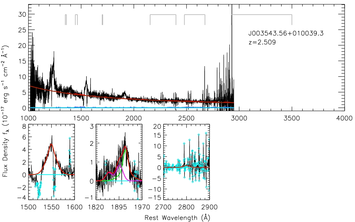
Here is the Quality Assessment (QA) plot of an example fit (this object 3586-55181-0956 is in DR9 but is replaced by 4221-55443-0830 in DR9Q).

Caption: Upper panel: continuum fit, where the brown line is the power-law continuum, the blue lines are the Fe II template, and the red lines are the pseudo-continuum. Bottom panels: emission line fits. The red lines are the total model, and the magenta line in the CIII] panel is Si III]+Al III. The cyan points are pixels that are masked out during the fit.

Error estimation: To estimate the uncertanities of compiled continuum and emission line properties from the multiple-component model fits, I used the Monte Carlo mock spectra method described in Shen et al. (2011) and Shen & Liu (2012). This method takes into account both statistical errors due to spectral noise and ambiguities in decomposing the lines. See these two papers for discussions on this method. I only used 10 mock spectra (instead of 50) in order to speed up the process.

The error estimation is still in progress (it takes 10 times longer than fitting the original ~87,800 spectra), so all the error terms are currently empty in the fits file. Will update it when this procedure is completed.

Caveats:

1. Continuum slope and flux amplitude are not accurate, due to the known flux calibration issue of BOSS quasars.
2. For a tiny fraction of objects (<<1%) the global continuum model is not a good prescription even if there is no BAL trough present. This is possibly caused by unusual intrinsic continuum shape, or data reduction problems. The conti_redchi2 will be large for these objects. As a result the emission line fit will fail too.
3. Objects with severe BAL troughs are often fit badly (both for continuum fits and emission line fits), albeit in many cases the fit seems OK (see the above example). The PCA results are probably better for these heavily absorbed objects.
4. The FeII emission around CIV is mostly constrained by wavelength regions up to MgII. Thus for a small number of high-z objects with only CIV coverage, the FeII template may be mismatched and may lead to incorrect power-law continuum level. For this reason, for 3422 objects with z_pipe>3.5 [i.e., no wavelength coverage beyond restframe ~2200A], the spectrum is fit without the UV Fe II template.
5. In very rare cases, the input systemic redshift [z_pipe] is very wrong, and as a result the spectral fit will fail. I plan to fix this for DR10 by using the visual inspection redshift [z_VI] as input systemic redshift.
6. Measurement errors not populated yet [see Error estimation].

Compiled properties: Gray entries were copied from DR9Q (Paris et al. 2012) and others are my measurements.

Important notes:

1. Why are these spectral fits needed as we already have the pipeline emission line fits? This is because the pipeline fits were using simple recipes for the local continuum and emission line, and usually do not provide accurate description of the line profile. However, in many cases we need to reproduce the line profile as closely as possible and get properties such as EW and FWHM right. This is crucial, for example, for computing virial BH mass estimates using broad line FWHM.
2. Input systemic redshifts [z_sys] are the pipeline redshifts [z_pipe], because the DR9Q catalog was not yet available when I started the fitting. Velocity offset and FWHMs are in units of km/s, EWs are in units of A, and fluxes are in units of erg/s/cm^2.
3. To select objects with good fits, I'd suggest to make a redchi2 cuts on both continuum fit and line fit (e.g., plot the distribution of redchi2, and cut at some threshold value, such as 0<redchi2<2). I'd also suggest to reject measurements where the errors are large (you will have to wait for the errors become available). But keep in mind that some very high S/N objects with large redchi2 could still be reasonable fits. If your sample is small, you should always check the QA plots for all objects in your sample.
4. All fits have QA plots, but unfortunately I don't have enough web space to host these files [3.5G gzipped]. If you have a small subsample and want to check how good the fits are, ask me for a gzipped file containing the QA plots for the subsample of quasars (should be less than 1000 objects).
5. Fluxes (continuum and line) are already scaled by 1+z_sys, so to compute luminosity, logL [erg/s]=logf + log(4*pi*d_L^2), where d_L is the luminosity distance computed using z_sys. Note that the continuum flux is already multiplied by restwavelength lambda.
6. To get power-law continuum luminosity at arbitrary rest wavelength lambda, simply do, logL_lambda [erg/s]= log[conti_fit[0]*(lambda/3000)^conti_fit[1]*1d-17*lambda*(1+z_sys)] + log(4*pi*d_L^2). However, the uncertainty of the continuum luminosity at arbitrary rest wavelength is not calculated using mock spectra. To estimate its uncertainty, you can use the reported errors in conti_fit[0] and conti_fit[1] and propagate errors assuming they are independent (this is an approximation because the errors in conti_fit[0] and conti_fit[1] are certainly correlated).
7. This global fitting recipe is different from the local fitting recipe in the value-added catalog in Shen et al. (2011, ApJS), but in most cases the difference is negligible. One noticeable difference is that CIV EW with the global fitting recipe is on average 0.06 dex larger than those in Shen et al. (2011) for the common DR7 quasars. Reasons for this difference: 1) I am fitting Fe II undernearth CIV for BOSS DR9 quasars, which lowers the power-law continuum [this effect contributes ~0.03 dex systematic offset in CIV EW]; 2) the difference between the global power-law continuum (i.e., more curved continuum undernearth CIV for the global fit) and the local power-law continuum fits [contributes another ~0.03 dex systematic offset in CIV EW]. Nevertheless, CIV FWHM is fully consistent with those in Shen et al. (2011) with a median offset of only 0.01 dex. Note that there is merit in both "local-continuum" and "global-continuum" fitting methods: the former eliminates bad global continuum fits in many objects, while the latter arguably provides a better estimate of the true continuum level undernearth the emission lines.
8. I tested fitting additional He II 1640 and OIII] 1663 emission and found their effect on CIV EW is negligible. This is because I am fitting CIV within [1500,1600], and the contribution from the bluewing of He II is not significant.
9. There are inevitably failed fits even if the spectrum looks OK, although such cases are rare. I have experimented ways to reduce junk fits as much as possible, but I can't gurantee that I have eliminated them all.
10. If you wish to use these fits to search for rare outliers with extreme spectral properties, please be advised that many of these outliers you find are most likely junk fits. So once again, you should check the QA plots for these "extreme" objects.

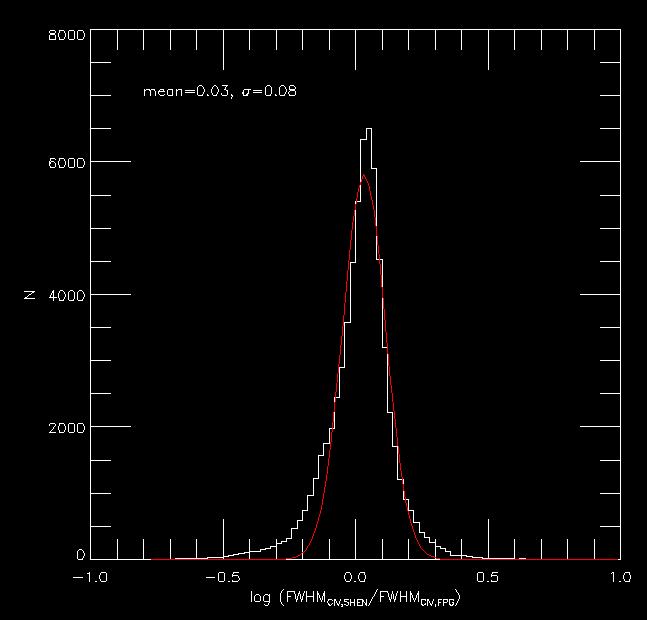
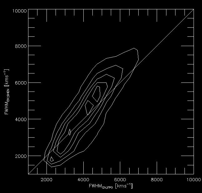
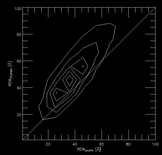
Comparison with the PCA results in Paris et al. (2012). I only compare CIV and MgII below, because CIII] is fitted in very different ways in both approaches.

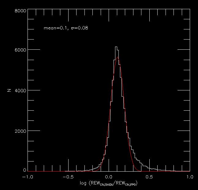
CIV: although generally the two sets of measurements are similar, there are some notable differences. The FWHMs have a slight tilt between my results and the PCA results. The CIV EW comparison also has a tilt, and on average the PCA results are ~0.1 dex lower than my results. We have investigated this discrepancy on CIV EW and here are the reasons: 1) the fits in Paris et al. (2012) is a similar "local-continuum" fit as in Shen et al. (2011), but the CIV EW was computed within the [1500,1600] window. While in Shen et al. (2011) the CIV EW was computed from the line model fit, which can extend beyond the [1500,1600] window. This causes a systematic ~0.04 dex underestimation of the CIV EWs in Paris et al. 2) The current fits depoly a "global-continuum" fit with Fe II around the CIV region. This introduces another ~0.06 dex average increase in CIV EW compared to those in Shen et al. (2011) [see Item 7 in "Important Notes" above]. Nevertheless, this ~0.1 dex offset is not crucial for most studies.

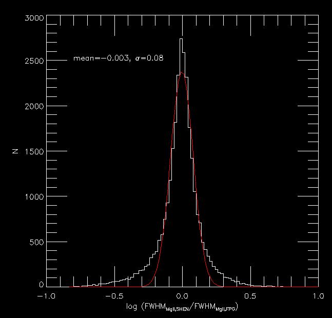
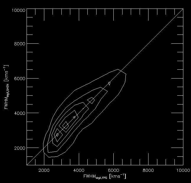
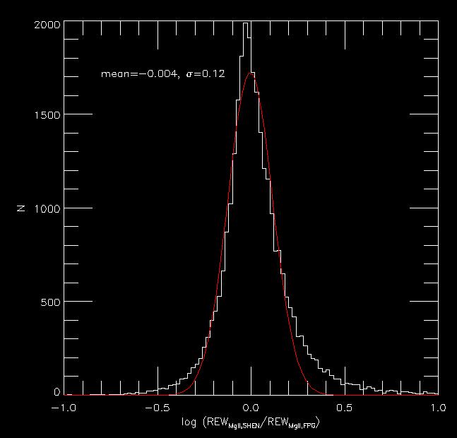
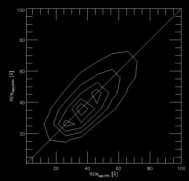
MgII: Both FWHMs and EWs seem to be in good agreement between the Paris et al. results and my measurements.

Some quick plots

Caption: Left: The CIV Baldwin effect. Right: CIV FWHM against CIII] FWHM from my fits. The two FWHMs are correlated with each other, consistent with the findings in Shen & Liu (2012). This correlation is much better than that of CIV FWHM versus MgII FWHM (or broad Balmer line FWHM).

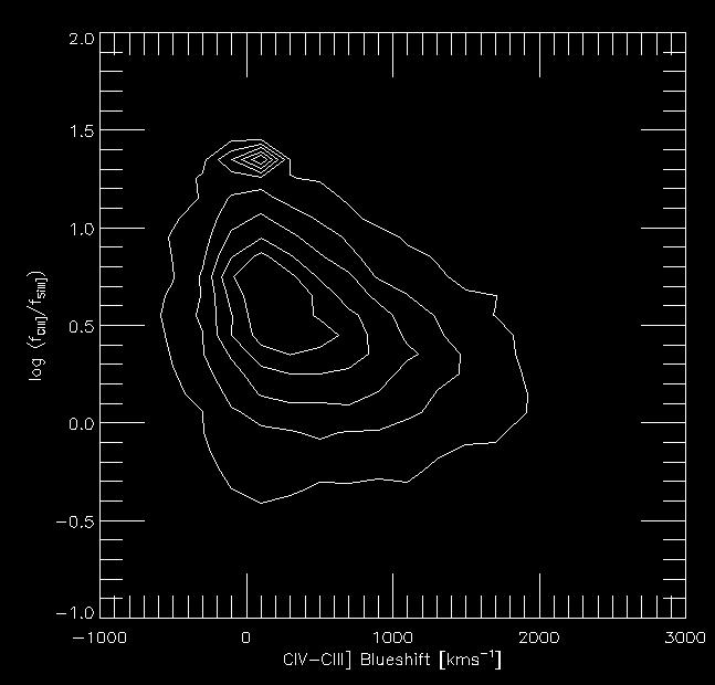
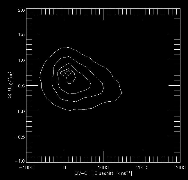
Caption: Flux ratio of CIII] to Si III] and Al III, as a function of CIV-CIII] blueshift. There is some indication that the relative flux ratio of Si III] and Al III to CIII] increases when CIV is more blueshifted (see Richards et al. 2011). In general the CIII]-MgII blueshift is much less than the CIV-MgII blueshift if the CIII] complex is decomposed properly.

Last modified: Sep 2012 by Yue Shen